This is a long-running project which I come back to and develop from time to time, and is now quite a large system of code which has gone through many iterations.
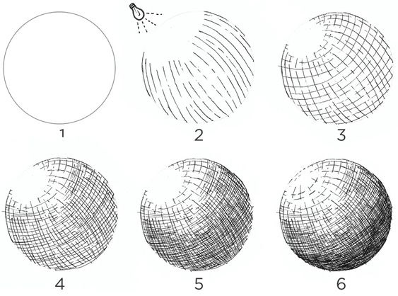
The aim for this project was to take in a source image or image sequence, and recreate it using a crosshatching effect where regions of different brightness are shaded in different ways, much like the below:
As with most of my creative coding projects, I wrote this one in java and Processing, though I used additional tools where needed, such as ffmpeg for rendering and Python for depth mapping (more on that later).
Here's an example render I made using stock footage:
And here’s what it looks like when each of the regions is shaded alone:
So how does it work?
We start by generating a set of particle fields. The particles in these fields have properties like velocity, colour, and size, which can each vary according to some rule if we choose. They move across the screen, new particles forming and old ones decaying.
Of course, if we were to draw all this to the screen, it would just be noise. To create a picture, we need to be selective about which ones we draw and when.
To do this, we take a source image and feed it into the code, which reads from it colour information (hue, saturation, brightness).
The trick is then to draw the particles only when certain brightness criteria are met. So if we have six particle fields, the first will always draw no matter what, the second requires that the source pixel underneath its particles have 17% brightness, the third 33% brightness… and so on.
There’s a lot more to it of course, but this is the basic idea.
Code Architecture
The basic code structure can be summed up with this diagram:
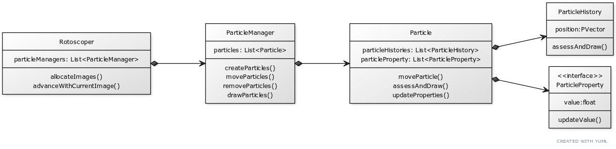
The Rotoscoper contains a list of ParticleManager objects, and is responsible for coordinating the sequence of events over the course of one frame update: from saving and loading images, to updating the particle fields and drawing to canvas.
There is one ParticleManager for each particle field. It contains a list of particle objects as well as field-level data (for example the brightness threshold required to draw). It is responsible for creating new particles, removing dead ones, updating the particles and drawing them.
Particles represent the sequences of dots you see onscreen. They contain methods for assessing whether they should be drawn and drawing of so, but otherwise act as wrappers for ParticleProperty and ParticleHistory objects.
The particles’ properties (colour, flow, size, etc.) are complex enough to be separated out into their own objects, connected via an interface ParticleProperty, to make handling groups of them straightforward. They are responsible for storing the property’s value and updating it according to the parameters of the algorithm.
Particle Histories - Each particle contains a list of the positions it has occupied during its journey, which are individually assessed against the current source frame to decide whether a point should be drawn (this is needed as the source frame might change, so we cannot guarantee a point drawn last frame should be drawn again this frame).
Challenges and Learnings
Performance and Memory
There were two big challenges associated with using the large numbers of particles required to achieve this effect.
First, performance. Dealing with a lot of particles means computing a lot of operations, which takes time. Processing only partially supports multithreading (anything involving drawing to canvas tends to blow up if multithreaded) but fortunately I was able to multithread most of the rest of the code; in particular the updating of particle positions and variables, and the saving and loading of frames can all be handled asynchronously. This was a learning experience as I’d never done multithreading before, and it made me consider carefully what was going on in my code and the required order of operations. I had to make extensive code changes such as building a new system of completion flags and logic to load and save images in a queue. But the experiment was successful, and I achieved something close to 10x performance gains (which I immediately squandered on making more particles, mwahahaha…).
Secondly, memory. My potato laptop struggled with creating enough lengthy arrays to hold all the particles. The solution here was simple - more disk, less RAM. I rewrote the code so that the particle managers can run one after the other in series, saving their particle field frames individually with transparency, so that the results can then be composited at the end to create the final frames.
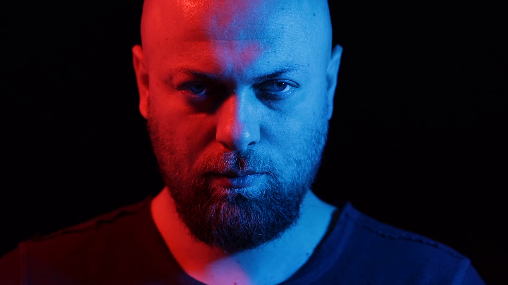
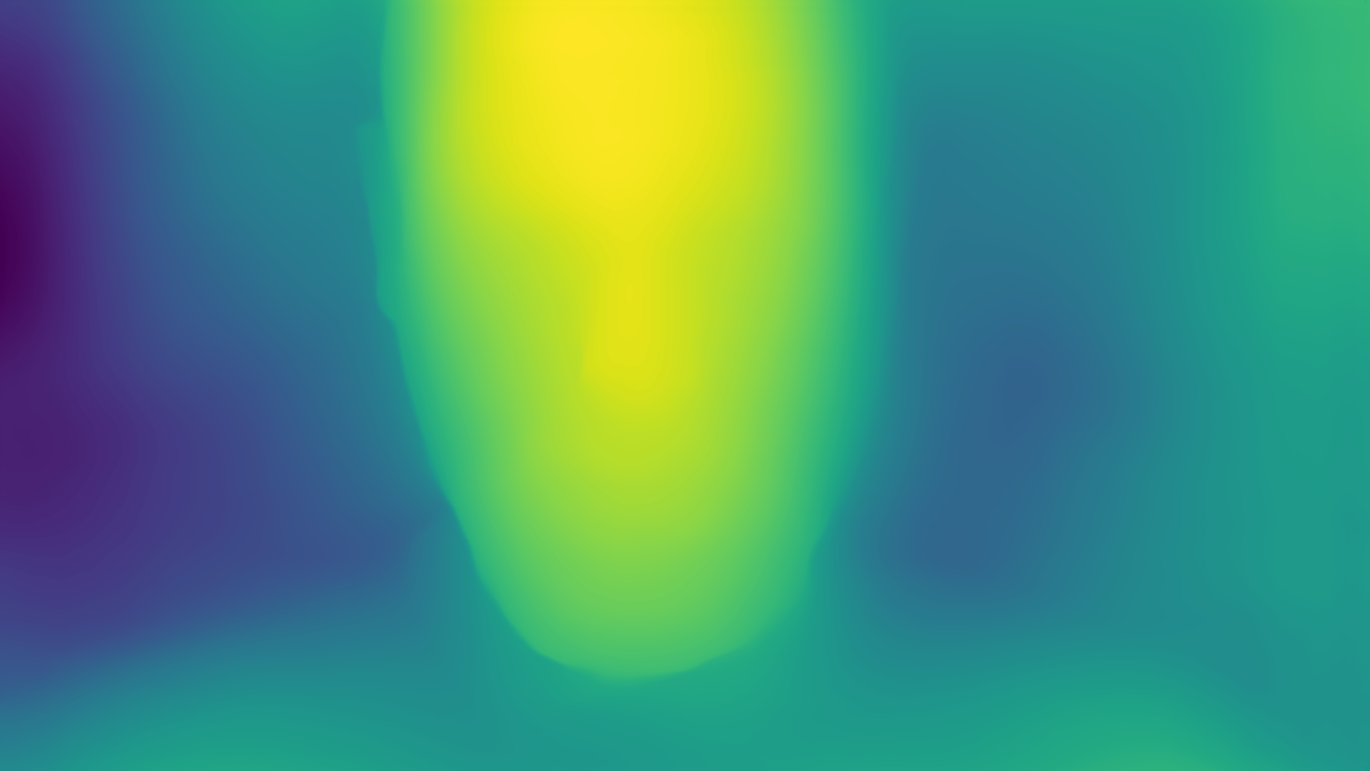
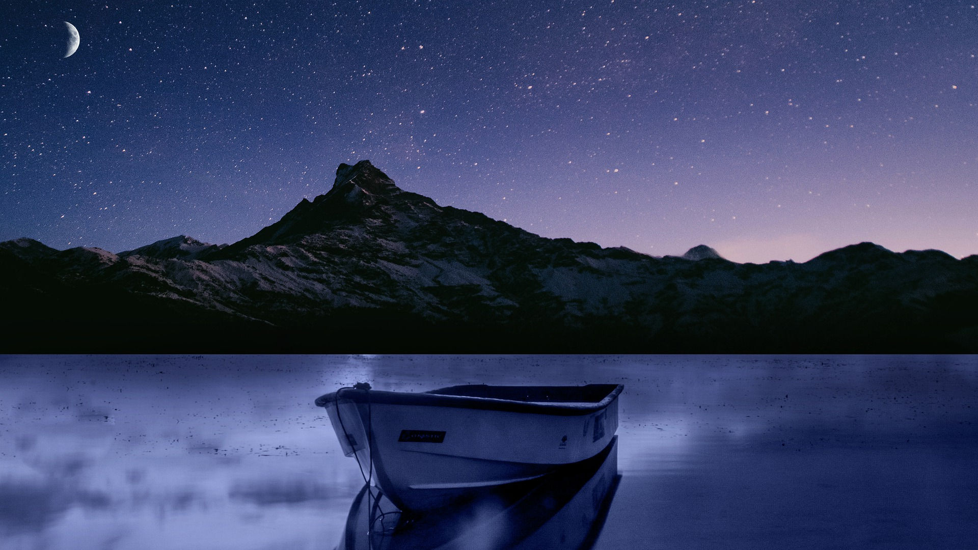
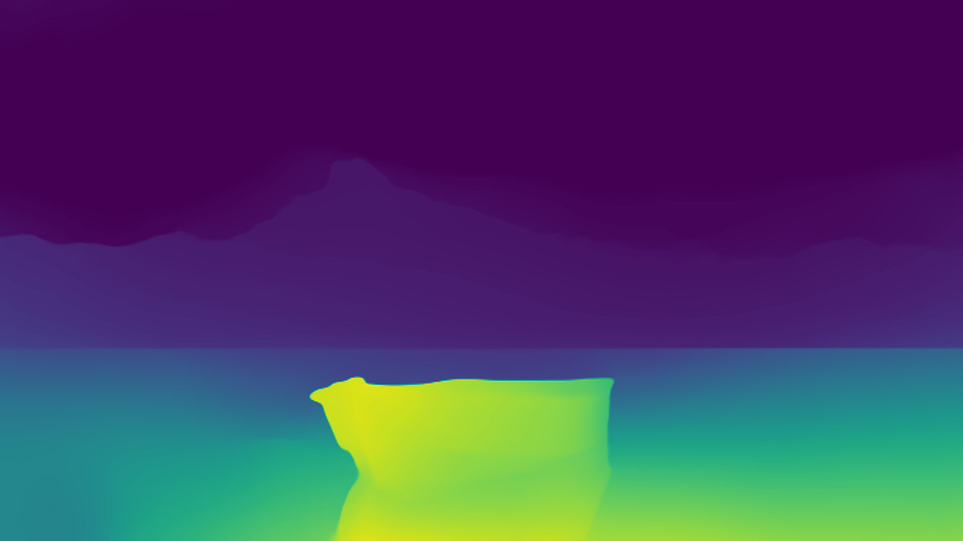
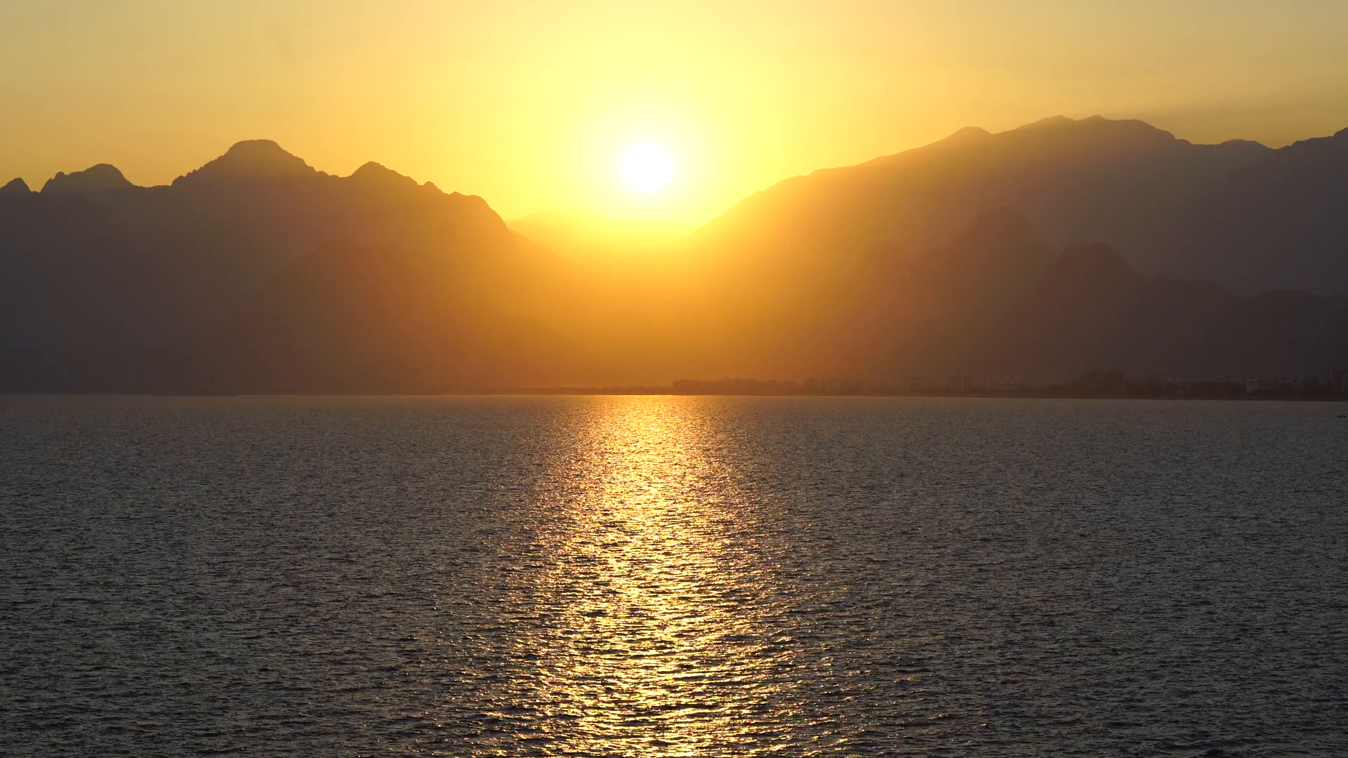
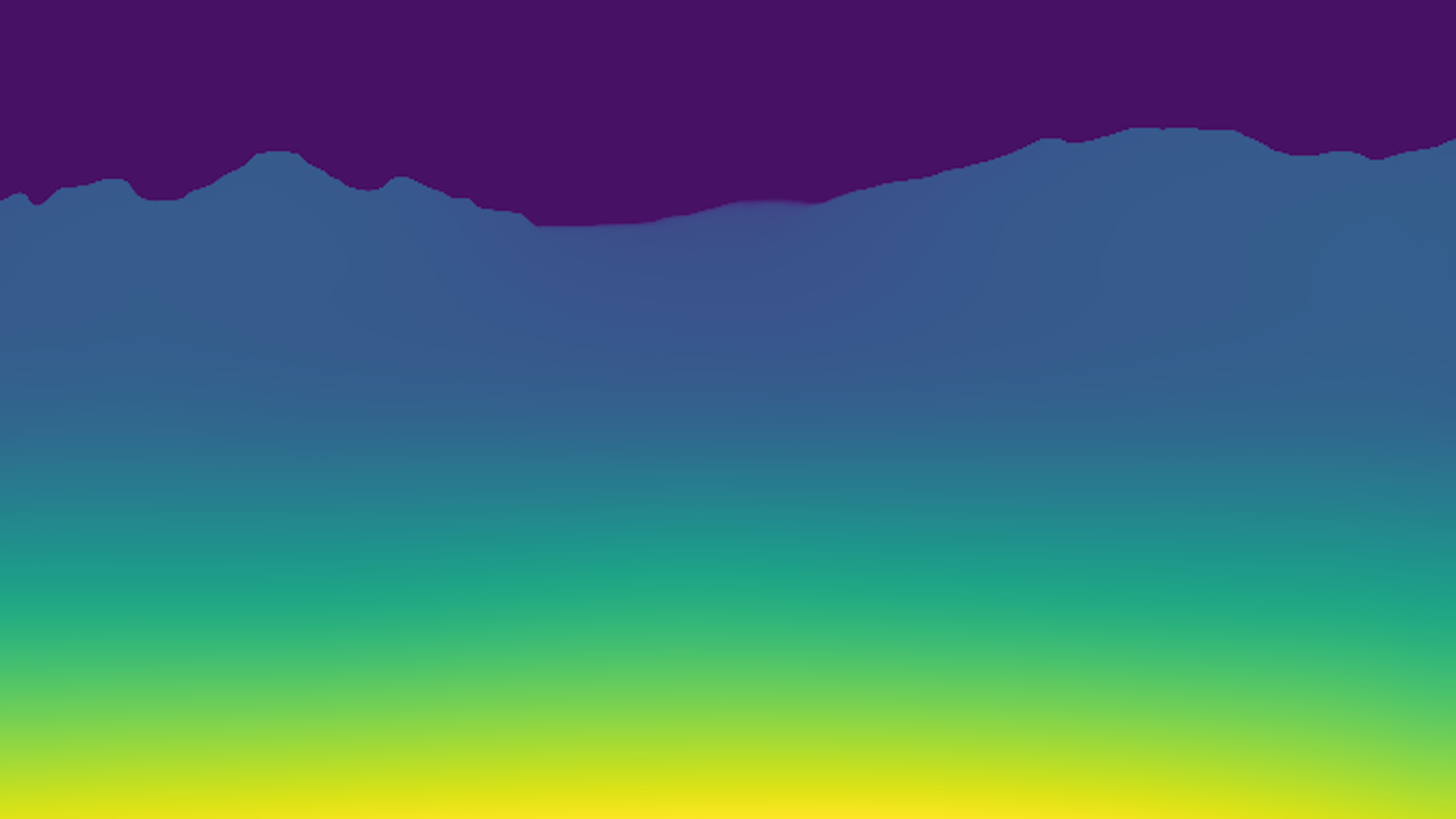
3D and Depth Mapping
I wanted to create a 3D effect, whereby the particles move more slowly and are smaller when further from the camera. Only… the information supplied to the algorithm is all in 2D. How to get around this? Well, there exist neural networks which can estimate depth from 2D images, rendering it as a heatmap, and it was a simple job to set up one of these in Python/Pytorch and then plug the result into my code to create a nice depth effect. The neural network approach isn’t perfect - the algorithm seems a little sensitive to small changes, which can create a flickering effect in the heatmap. But the results are decent enough for our purposes:
Generative Flow Patterns
I also wanted to create more interesting flow patterns for the particle fields. Initially these were just simple rules, for example having the particles in a region all move in the same fixed direction, or having them move in spirals. But my favourite flows are generative - that is, they depend on other features of the particle, or on features of the source image. For example, in the following render, the particles' direction depends on the hue and saturation of the source pixel, producing an interesting texture.
Colour
What colour should the particles be? A simple answer would be to sample the source image colour underneath the particle and use this as the particle’s colour, but this tends to result in boring images which seem too keen to replicate the source without adding anything interesting.
In general, the colour can be a function of anything, (H’,S’,B’) = f(H,S,B,t,P), where H’,S’,B’ are particle hue, saturation and brightness, H,S,B are the same for the source pixel, t is time, and P is a vector of the particle’s properties (speed, velocity etc.). With this very general schema, it’s possible to imagine many different ways to assign colour to a particle. The ColourMapper class and ColourMappingFunction enum exist to control this colour generation.
There’s another step to this, however. I found that the images looked much more interesting when the particle fields could each have two colour mappers with different rules and parameters, which are then mixed according to a mixing rule and coefficient. This allows the creation of endless combinations of colour schemes, especially when you consider that each particle field in the drawing can have its own colour setup. The next example shows an oscillating colour scheme, where hue depends on source hue but also on time:
Change over time
What if we want our values to change over time? The ParamModifier abstract class exists to create smooth transitions between different parameter values. The concrete classes come in different forms depending on how we want the parameters to vary (linear, exponential decay, and so on).
In the case of numerical parameters, these assign the parameter a value which is a weighted average of the starting and target values - starting by favouring the starting value and slowly starting to favour the target, so as to produce a smooth transition. For non-numerical parameters such as FlowType (an enum), the process is much the same, though it is the downstream consequences of the non-numerical parameter's value (in this case the computed flow step) which must be combined during the transition. The following video contains a typical transition between different flow patterns:
Gaussians, Gaussians and more Gaussians!
Just a little note, but I have inherited from my physics degree a love of Gaussian distributions, and find they are useful in almost any circumstance. I could, for example, have made all the particles in a given flow field move at the same speed, but this tends to produce a flat and unsatisfying picture. You get much nicer results when the values are sampled from a distribution, meaning the parameters we set are the mean and width of that distribution, rather than setting the speed values directly.
And we'll end on some dancing: